Classification: Predicting Wheat Variety Using Ensemble Models
Goal
The project’s goal is to accurately predict the wheat variety (Kama, Rosa, Canadian) using the attributes corresponding to each of the wheat variety. Additionally, it will be interesting to know which of the features play an important role in predicting the accurate wheat variety.
Data
In this project, I classify wheat variety based on the wheat kernel’s geometrical properties. There are three varieties of wheat (Kama, Rosa, and Canadian), which is the categorical variable. Each variety has 70 observations accounting for a total of 210 observations. There are seven features (X), including area, perimeter, compactness, length of the kernel, width of the kernel, asymmetry coefficient, and length of kernel groove. Data are collected from UC Irvine Machine Learning Repository at https://archive-beta.ics.uci.edu/ml/datasets/seeds.
Data Preprocessing
library(dplyr)
wht_data <- read.csv("wheat_var_data.csv")
glimpse(wht_data)
## Rows: 210
## Columns: 8
## $ area <dbl> 15.26, 14.88, 14.29, 13.84, 16.14, 14.38, 14.69, …
## $ perimeter <dbl> 14.84, 14.57, 14.09, 13.94, 14.99, 14.21, 14.49, …
## $ compactness <dbl> 0.8710, 0.8811, 0.9050, 0.8955, 0.9034, 0.8951, 0…
## $ length_kernel <dbl> 5.763, 5.554, 5.291, 5.324, 5.658, 5.386, 5.563, …
## $ width_kernel <dbl> 3.312, 3.333, 3.337, 3.379, 3.562, 3.312, 3.259, …
## $ asymmetry_coef <dbl> 2.2210, 1.0180, 2.6990, 2.2590, 1.3550, 2.4620, 3…
## $ length_kernel_groove <dbl> 5.220, 4.956, 4.825, 4.805, 5.175, 4.956, 5.219, …
## $ wheat_variety <int> 1, 1, 1, 1, 1, 1, 1, 1, 1, 1, 1, 1, 1, 1, 1, 1, 1…summary(wht_data)## area perimeter compactness length_kernel
## Min. :10.59 Min. :12.41 Min. :0.8081 Min. :4.899
## 1st Qu.:12.27 1st Qu.:13.45 1st Qu.:0.8569 1st Qu.:5.262
## Median :14.36 Median :14.32 Median :0.8734 Median :5.524
## Mean :14.85 Mean :14.56 Mean :0.8710 Mean :5.629
## 3rd Qu.:17.30 3rd Qu.:15.71 3rd Qu.:0.8878 3rd Qu.:5.980
## Max. :21.18 Max. :17.25 Max. :0.9183 Max. :6.675
## width_kernel asymmetry_coef length_kernel_groove wheat_variety
## Min. :2.630 Min. :0.7651 Min. :4.519 Min. :1
## 1st Qu.:2.944 1st Qu.:2.5615 1st Qu.:5.045 1st Qu.:1
## Median :3.237 Median :3.5990 Median :5.223 Median :2
## Mean :3.259 Mean :3.7002 Mean :5.408 Mean :2
## 3rd Qu.:3.562 3rd Qu.:4.7687 3rd Qu.:5.877 3rd Qu.:3
## Max. :4.033 Max. :8.4560 Max. :6.550 Max. :3By inspecting mean and median of all seven attributes, one can conclude that there are no outliers/anomalies. Also, we need to convert the wheat_variety variable into categorical or qualitative or class variable instead of an integer.
library(dplyr)
wht_data$wheat_variety <- as.factor(wht_data$wheat_variety)
wht_data <- wht_data %>%
  mutate(wheat_var =
           ifelse(wheat_variety == "1", "Kama",
                  ifelse(wheat_variety == "2", "Rosa", "Canadian"))) %>%
  select(-wheat_variety)
str(wht_data)
## 'data.frame': 210 obs. of 8 variables:
## $ area : num 15.3 14.9 14.3 13.8 16.1 ...
## $ perimeter : num 14.8 14.6 14.1 13.9 15 ...
## $ compactness : num 0.871 0.881 0.905 0.895 0.903 ...
## $ length_kernel : num 5.76 5.55 5.29 5.32 5.66 ...
## $ width_kernel : num 3.31 3.33 3.34 3.38 3.56 ...
## $ asymmetry_coef : num 2.22 1.02 2.7 2.26 1.35 ...
## $ length_kernel_groove: num 5.22 4.96 4.83 4.8 5.17 ...
## $ wheat_var : chr "Kama" "Kama" "Kama" "Kama" ...Exploratory Data Analysis
Let us now look at the relationships of the three wheat varieties with each of the seven features.
library(dplyr)
wht_data %>%
  group_by(wheat_var) %>%
  summarise_all(mean)
## # A tibble: 3 × 8
## wheat_var area perimeter compactness length_kernel width_kernel
## <chr> <dbl> <dbl> <dbl> <dbl> <dbl>
## 1 Canadian 11.9 13.2 0.849 5.23 2.85
## 2 Kama 14.3 14.3 0.880 5.51 3.24
## 3 Rosa 18.3 16.1 0.884 6.15 3.68
## # … with 2 more variables: asymmetry_coef <dbl>, length_kernel_groove <dbl>On average, Rosa wheat variety seem to have higher length, width, area, perimeter and compactness, followed by Kama variety. However, Canadian variety has the highest average asymmetry coefficient compared with other wheat varieties.
library(ggplot2)
library(geomtextpath)

ggplot(wht_data, aes(x = length_kernel, colour = wheat_var, label = wheat_var)) +
  geom_textdensity(size = 6, fontface = 2, hjust = 0.2, vjust = 0.3) +
  theme(legend.position = "none") + theme_bw()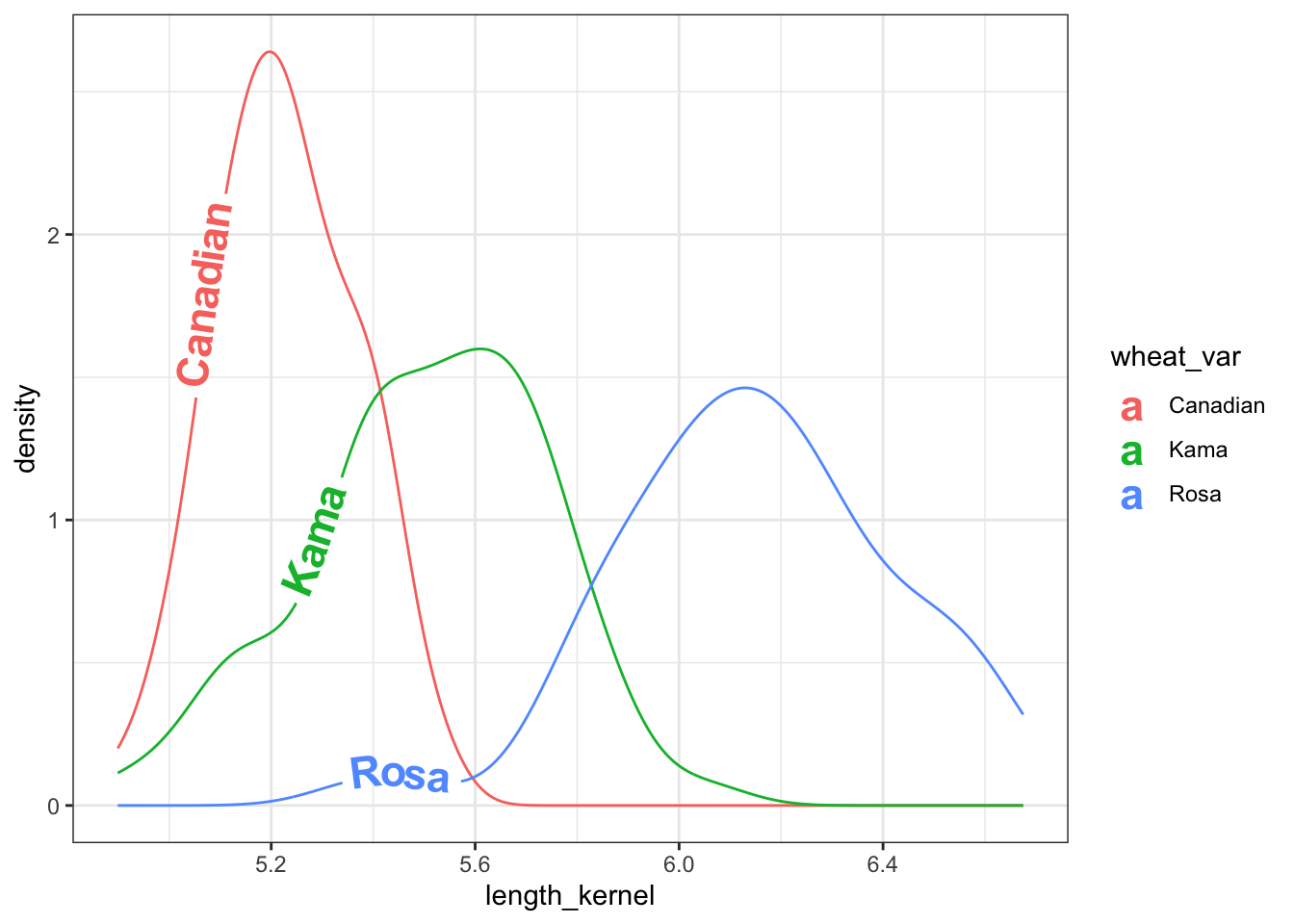
Figure 1: Density plot of kernel length of three wheat varieties
library(ggplot2)
library(geomtextpath)
ggplot(wht_data, aes(x = asymmetry_coef, colour = wheat_var,
                     label = wheat_var)) +
       theme(legend.position = "none") +
       geom_textdensity(size = 6, fontface = 2, spacing = 50,
                   vjust = -0.2, hjust = "ymax") + ylim(c(0, 0.4)) + theme_minimal()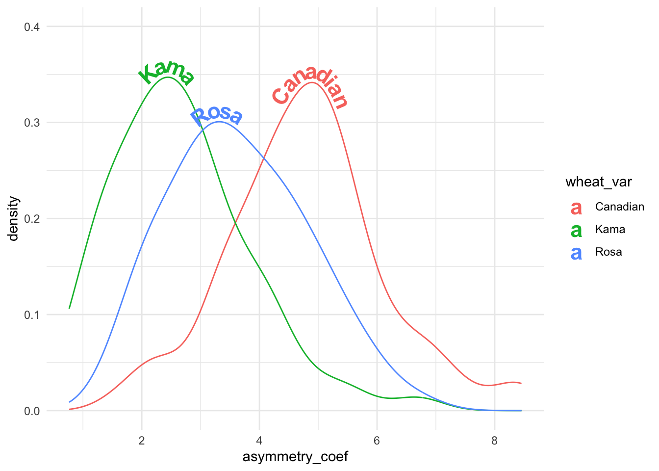
Figure 2: Density plot of asymmetry coefficient of three wheat varieties
ggplot(wht_data, aes(x = length_kernel, y = width_kernel,
                     color = wheat_var)) +
  geom_point(alpha = 0.3) + theme(legend.position = "bottom") +
  geom_labelsmooth(aes(label = wheat_var), text_smoothing = 30,
                   fill = "#F6F6FF",
                method = "loess", formula = y ~ x,
                size = 4, linewidth = 1, boxlinewidth = 0.3) +
  scale_colour_manual(values = c("forestgreen", "deepskyblue4", "tomato4")) +
   theme_bw()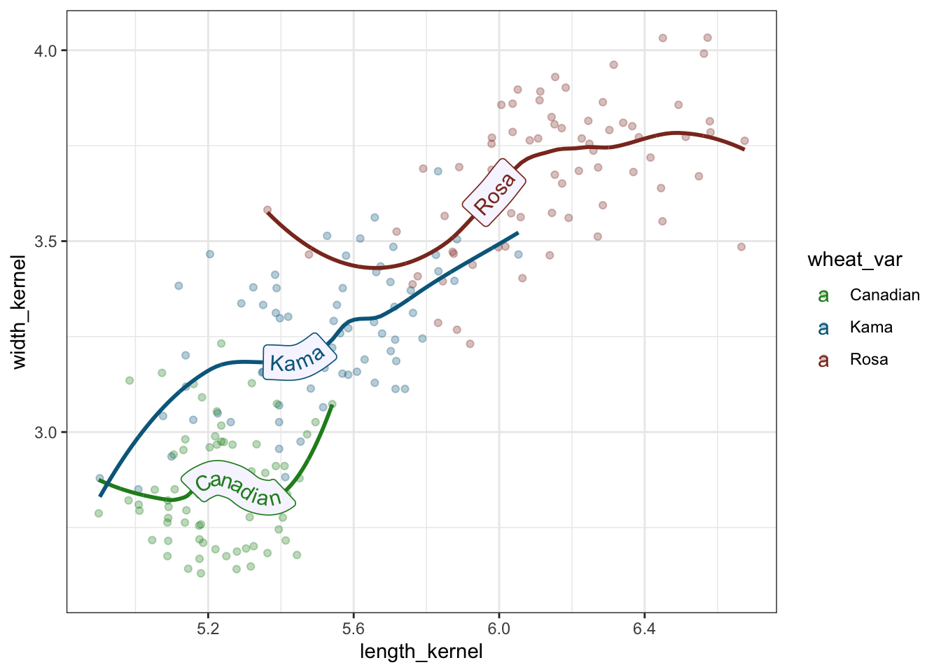
Figure 3: Trend Lines through scatter plot of length and width of wheat varieties
Correlation Pairs
The correlation plot shown below reveal that there is multicollinearity problem. To deal with multicollinearity, there are a couple of solutions, including 1) removing one of the features from the highly correlated feature combinations, 2) linearly combine the variables using principal component analysis or partial least squares. In this case, I will use the first option to remove perimeter, length_kernel, and width_kernel features.
library(psych)
pairs.panels(wht_data)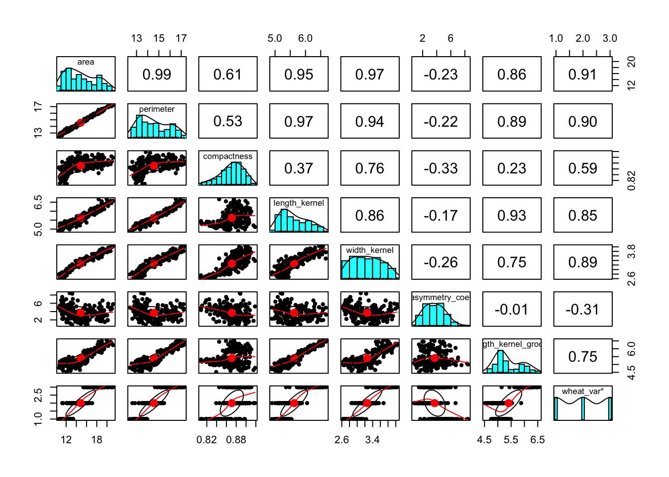
The correlation pairs plot after removing the above mentioned features is shown below.
library(psych)
library(tidyverse)
wht_data <- wht_data %>%
  select(!c(perimeter, length_kernel, width_kernel))

pairs.panels(wht_data)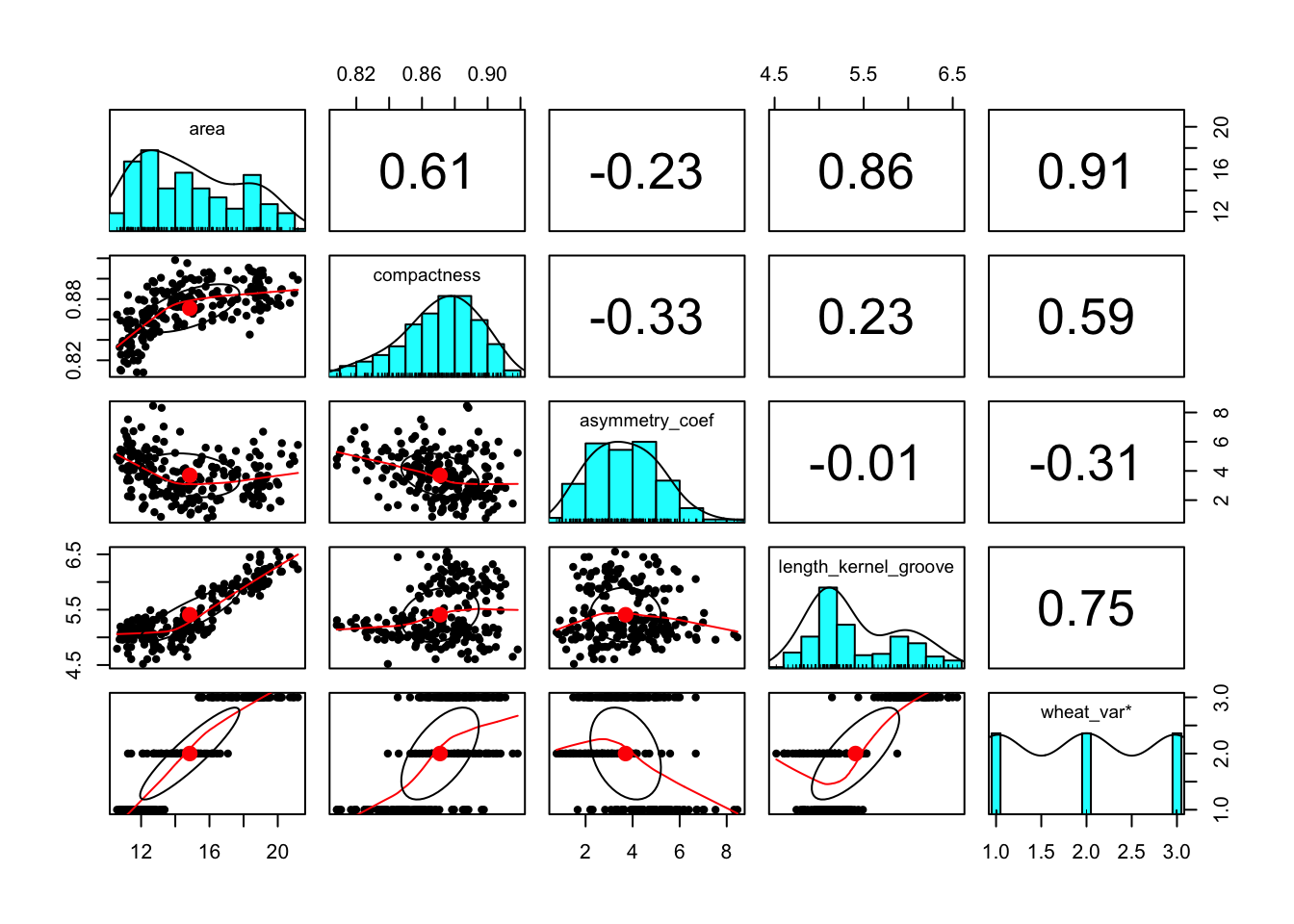
Near-zero variance features
library(caret)
near_0_var <- nearZeroVar(wht_data, names = TRUE)
print(near_0_var)
## character(0)The result indicate that there are no zero variance features, which is good. Therefore, we can use all the features to predict the the class of wheat variety.
Checking for class imbalance
It was already known that there are equal observations for each of the wheat varieties in our dataset. That is, each variety has 70 observations for a total of 210 observations. Therefore, our data set do not suffer with class imbalance problem.
table(wht_data$wheat_var)##
## Canadian Kama Rosa
## 70 70 70Ensemble Models
Splitting the data
library(caret)

set.seed(4321)
wht_data$wheat_var <- as.factor(wht_data$wheat_var)
in_train <- createDataPartition(y = wht_data$wheat_var,
                                p = 0.80, list = FALSE)

training <- wht_data[in_train,]
testing <- wht_data[-in_train,]

table(training$wheat_var)
##
## Canadian Kama Rosa
## 56 56 56table(testing$wheat_var)##
## Canadian Kama Rosa
## 14 14 14head(training)## area compactness asymmetry_coef length_kernel_groove wheat_var
## 2 14.88 0.8811 1.018 4.956 Kama
## 3 14.29 0.9050 2.699 4.825 Kama
## 4 13.84 0.8955 2.259 4.805 Kama
## 5 16.14 0.9034 1.355 5.175 Kama
## 7 14.69 0.8799 3.586 5.219 Kama
## 8 14.11 0.8911 2.700 5.000 Kamastr(training)## 'data.frame': 168 obs. of 5 variables:
## $ area : num 14.9 14.3 13.8 16.1 14.7 ...
## $ compactness : num 0.881 0.905 0.895 0.903 0.88 ...
## $ asymmetry_coef : num 1.02 2.7 2.26 1.35 3.59 ...
## $ length_kernel_groove: num 4.96 4.83 4.8 5.17 5.22 ...
## $ wheat_var : Factor w/ 3 levels "Canadian","Kama",..: 2 2 2 2 2 2 2 2 2 2 ...Hyperparameter Tuning
In the case of Random Forest model, number of features selected in mtry for constructing decision trees (or more specifically at each split) is probably the most important tuning parameter.
Random Search for Randomly Selecting Predictors (mtry)
#modelLookup("rf")

library(caret)

fitControl <- trainControl(method = "repeatedcv",
                            number = 5, repeats = 5,
                           search = 'random')

#manual_grid_rf <- expand.grid(#n.trees = c(100, 200, 500, 750, 1000),
#                         #interaction.depth = c(1, 4, 6),
#                         #shrinkage = 0.1,
#                         #n.minobsinnode = 10,
#                         .mtry = c(1:5))
set.seed(143)
library(tictoc)
tic()

model_rf_random <- train(wheat_var ~.,
                         data = training,
                         method = "rf",
                         metric = 'Accuracy',
                         trControl = fitControl,
                         verbose = FALSE,
                         tuneLength = 4)
toc()
## 3.158 sec elapsedprint(model_rf_random)## Random Forest
##
## 168 samples
## 4 predictor
## 3 classes: 'Canadian', 'Kama', 'Rosa'
##
## No pre-processing
## Resampling: Cross-Validated (5 fold, repeated 5 times)
## Summary of sample sizes: 134, 134, 135, 135, 134, 135, ...
## Resampling results across tuning parameters:
##
## mtry Accuracy Kappa
## 1 0.9357494 0.9035902
## 4 0.9250522 0.8875511
##
## Accuracy was used to select the optimal model using the largest value.
## The final value used for the model was mtry = 1.plot(model_rf_random)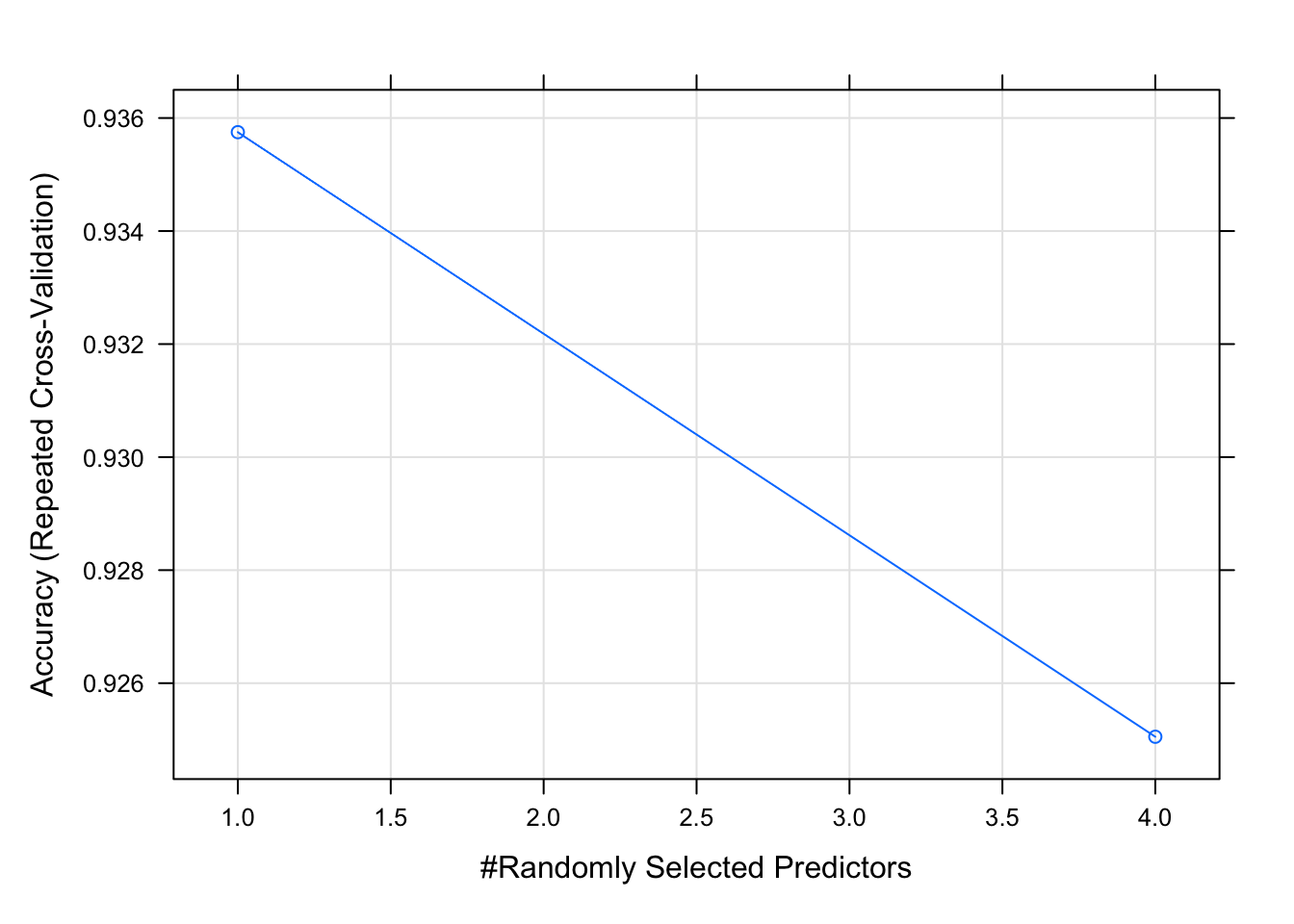
Grid Search for Selecting Optimal mtry
fitControl <- trainControl(method = "repeatedcv",
                            number = 3, repeats = 5,
                           search = 'grid')

tunegrid <- expand.grid(.mtry = (1:4))

model_rf_grid <- train(wheat_var ~.,
                       data = training,
                       method = 'rf',
                       metric = 'Accuracy',
                       tuneGrid = tunegrid)
print(model_rf_grid)
## Random Forest
##
## 168 samples
## 4 predictor
## 3 classes: 'Canadian', 'Kama', 'Rosa'
##
## No pre-processing
## Resampling: Bootstrapped (25 reps)
## Summary of sample sizes: 168, 168, 168, 168, 168, 168, ...
## Resampling results across tuning parameters:
##
## mtry Accuracy Kappa
## 1 0.9247728 0.8865813
## 2 0.9224229 0.8830108
## 3 0.9205031 0.8800244
## 4 0.9187102 0.8773807
##
## Accuracy was used to select the optimal model using the largest value.
## The final value used for the model was mtry = 1.plot(model_rf_grid)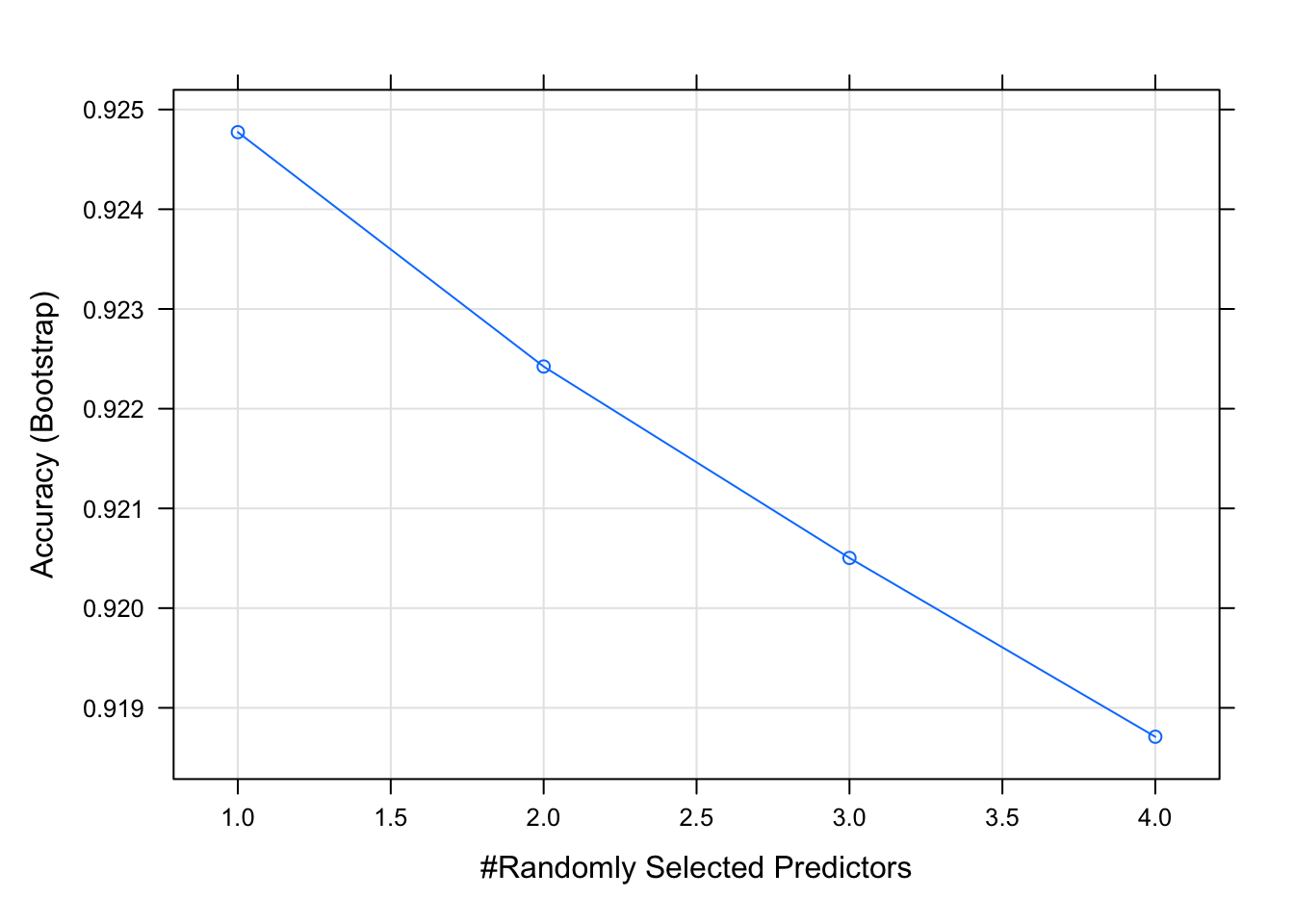
The grid search and random search suggest same mtry values in this case. Generally, grid search is considered as accurate as it evaluates all the combinations in the proposed Cartesian grid. Therefore, for modeling random forest model, mtry = 1 was used for the final model (shown later).
library(caret)
manual_grid <- expand.grid(n.trees = c(100, 200, 500),
                         interaction.depth = c(1, 4, 6),
                         shrinkage = 0.1,
                         n.minobsinnode = 10)

fitControl <- trainControl(method = "repeatedcv",
                            number = 3, repeats = 5)
library(tictoc)
tic()
set.seed(123)
model_gbm_grid <- train(wheat_var ~.,
                         data = training,
                         method = "gbm",
                         trControl = fitControl,
                         verbose = FALSE,
                         tuneGrid = manual_grid)
toc()
## 6.457 sec elapsedplot(model_gbm_grid)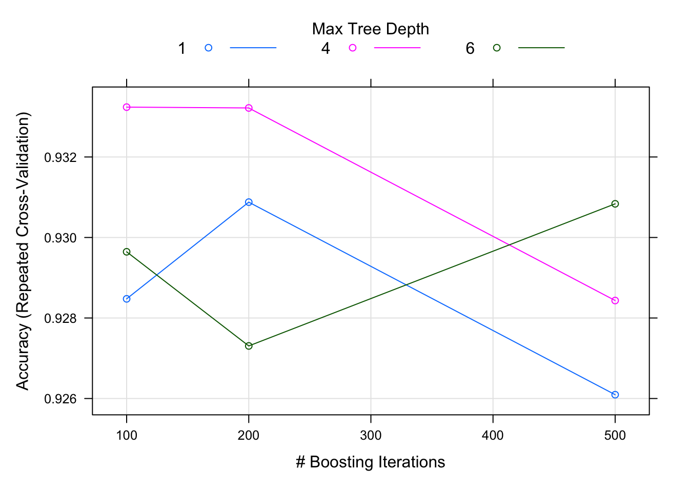
plot(model_gbm_grid,
     metric = "Kappa",
     plotType = "level")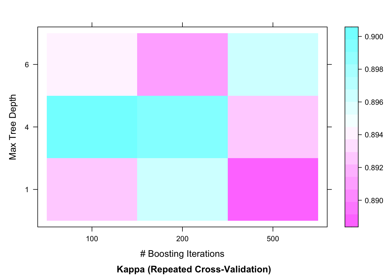
The plots of gradient boosting model reveal that maximum accuracy is achieved when the number of trees are set at 100 with the tree depth (interaction.depth) at 4.
Classification: Random Forest
### load the randomForest package
library(randomForest)
set.seed(123)
### train the random forest model: model_rf
model_rf <- randomForest(formula = wheat_var ~.,
                         data = training,
                         ntree = 300,
                         mtry = 1)

### print the rf model
print(model_rf)
##
## Call:
## randomForest(formula = wheat_var ~ ., data = training, ntree = 300, mtry = 1)
## Type of random forest: classification
## Number of trees: 300
## No. of variables tried at each split: 1
##
## OOB estimate of error rate: 7.14%
## Confusion matrix:
## Canadian Kama Rosa class.error
## Canadian 52 4 0 0.07142857
## Kama 6 50 0 0.10714286
## Rosa 0 2 54 0.03571429### variable importance plots
varImpPlot(model_rf)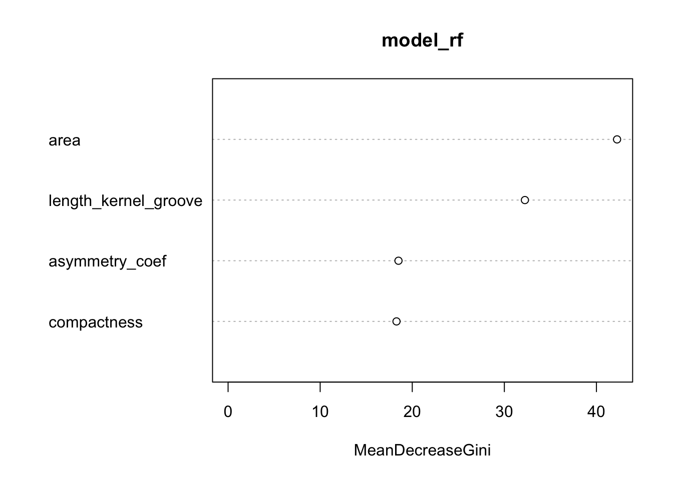
print(model_rf$importance)## MeanDecreaseGini
## area 42.23948
## compactness 18.28924
## asymmetry_coef 18.50317
## length_kernel_groove 32.23213Classification : Gradient Boosting Model
### load the gradient boosting model package
library(gbm)
set.seed(143)
### train the gradient boosting model: model_gbm
model_gbm <- gbm(formula = wheat_var ~.,
                         data = training,
                         n.trees = 100,
                         interaction.depth = 4,
                         shrinkage = 0.1,
                         n.minobsinnode = 10)
## Distribution not specified, assuming multinomial ...### print the gbm model
print(model_gbm)## gbm(formula = wheat_var ~ ., data = training, n.trees = 100,
## interaction.depth = 4, n.minobsinnode = 10, shrinkage = 0.1)
## A gradient boosted model with multinomial loss function.
## 100 iterations were performed.
## There were 4 predictors of which 4 had non-zero influence.### summarize gbm's variable importance plots
summary(model_gbm)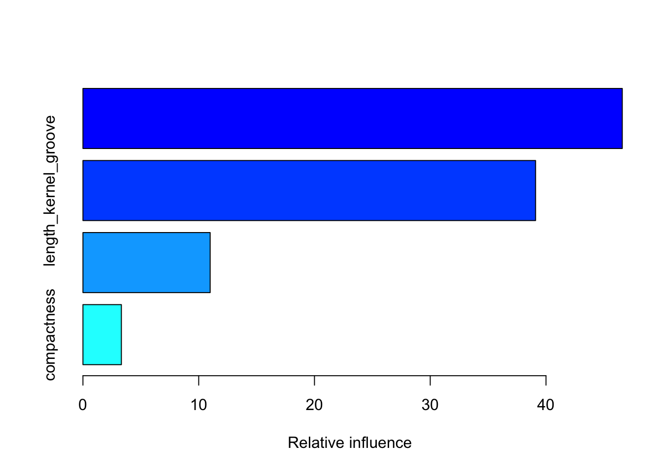
##                                       var   rel.inf
## area                                 area 46.589280
## length_kernel_groove length_kernel_groove 39.100031
## asymmetry_coef             asymmetry_coef 10.990146
## compactness                   compactness  3.320543
Evaluating both Random Forest and Gradient Boosting Algorithms
library(Metrics)

preds_rf <- predict(model_rf, newdata = testing)
preds_gbm <- predict(model_gbm, n.trees = 100, newdata = testing, type = "response")
## compute confusion matrix


classes <- colnames(preds_gbm)[apply(preds_gbm, 1, which.max)]
result_gbm <- data.frame(testing$wheat_var, classes)

#print(result_gbm)
(cm_rf <- confusionMatrix(preds_rf, testing$wheat_var))
## Confusion Matrix and Statistics
##
## Reference
## Prediction Canadian Kama Rosa
## Canadian 13 0 0
## Kama 1 12 0
## Rosa 0 2 14
##
## Overall Statistics
##
## Accuracy : 0.9286
## 95% CI : (0.8052, 0.985)
## No Information Rate : 0.3333
## P-Value [Acc > NIR] : 8.716e-16
##
## Kappa : 0.8929
##
## Mcnemar's Test P-Value : NA
##
## Statistics by Class:
##
## Class: Canadian Class: Kama Class: Rosa
## Sensitivity 0.9286 0.8571 1.0000
## Specificity 1.0000 0.9643 0.9286
## Pos Pred Value 1.0000 0.9231 0.8750
## Neg Pred Value 0.9655 0.9310 1.0000
## Prevalence 0.3333 0.3333 0.3333
## Detection Rate 0.3095 0.2857 0.3333
## Detection Prevalence 0.3095 0.3095 0.3810
## Balanced Accuracy 0.9643 0.9107 0.9643(cm_gbm <- confusionMatrix(as.factor(classes), testing$wheat_var))## Confusion Matrix and Statistics
##
## Reference
## Prediction Canadian Kama Rosa
## Canadian 13 0 0
## Kama 1 12 0
## Rosa 0 2 14
##
## Overall Statistics
##
## Accuracy : 0.9286
## 95% CI : (0.8052, 0.985)
## No Information Rate : 0.3333
## P-Value [Acc > NIR] : 8.716e-16
##
## Kappa : 0.8929
##
## Mcnemar's Test P-Value : NA
##
## Statistics by Class:
##
## Class: Canadian Class: Kama Class: Rosa
## Sensitivity 0.9286 0.8571 1.0000
## Specificity 1.0000 0.9643 0.9286
## Pos Pred Value 1.0000 0.9231 0.8750
## Neg Pred Value 0.9655 0.9310 1.0000
## Prevalence 0.3333 0.3333 0.3333
## Detection Rate 0.3095 0.2857 0.3333
## Detection Prevalence 0.3095 0.3095 0.3810
## Balanced Accuracy 0.9643 0.9107 0.9643Conclusions
The ensemble models suggest that there is an accuracy of about 93% in case of both Random Forest and GBM predicting the correct wheat variety using a set of features. Variable importance plot results of both the models show that area (highest importantance), length of kernel groove, asymmetry coefficient, and compactness (lowest importance) play an important role in wheat variety prediction. in case of both the models. Overall, both the models show consistent results and agree with each other.
In the UC Irvine’s data repository, it was indicated that there was some critical features that they could not provide due to proprietary issues associated with those data. Therefore, given those additional features, there is a scope for improving accuracy rate. Overall, the classification results show that accuracy of predicting the correct wheat variety is high.